Introduction

The past few weeks at Overworld, we’ve been heads down shipping. Waypoint 1 was our largest public drop in a while. It’s a new playable world model, representing a massive jump in interactivity and significantly reduced latency compared to other models in the space. Furthermore, it build a foundation for us to have a much faster research cadence as we move forward.

We’re returning to weekly technical blog posts, just like the early OWL days. During Waypoint 1 pretraining, we ran a large number of experiments simultaneously. Some of these made it into the released model, many didn’t, and a few changed how we approach building world models as a whole. Rather than letting these results stay buried in internal notes and W&B runs, we’re going to be sharing them regularly through our blog.

This week, we’re diving back into our continued work on Diffusion Autoencoders, a diffusion-based alternative to traditional GAN autoencoders. While these models did not make into Waypoint 1, the results were too strong and directionally important to ignore. What started as a simple experiment quickly turned into us reassessing how compression and diffusion training should fit together.

Today we’re going to walk through what we tried, what we broke, what worked and why we believe diffusion tokenizers represent a higher ceiling for world models.

Autoencoders Once More

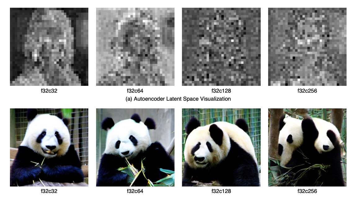
We have talked about autoencoders many times in the past. In summary, a latent space being diffusable is generally equivalent to it being image-like. Understanding this serves as important context for further sections of this blog post. What we mean by having image-like latents, is that the spectral and spatial composition of a latent should correspond with the spectral and spatial composition of the original image. The top left of the latent should be representing the top left of the image, the high frequency features of the latent should represent the high frequency features of the image, and so-on. Autencoders that skirt these principles can give high quality reconstructions but suffer when it comes to generation. High channel counts are shown to do this in the DCAE 1.5 paper:

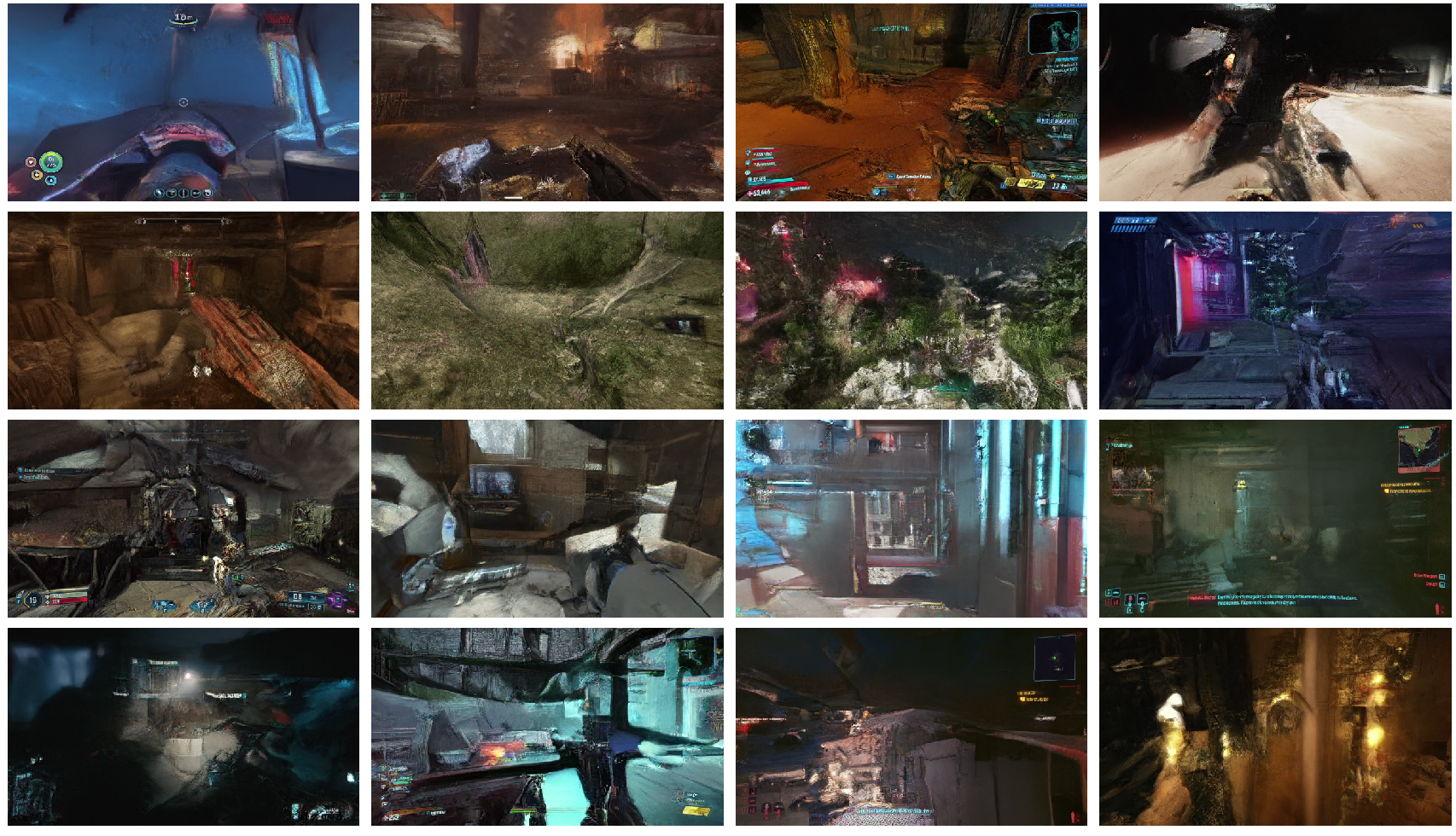
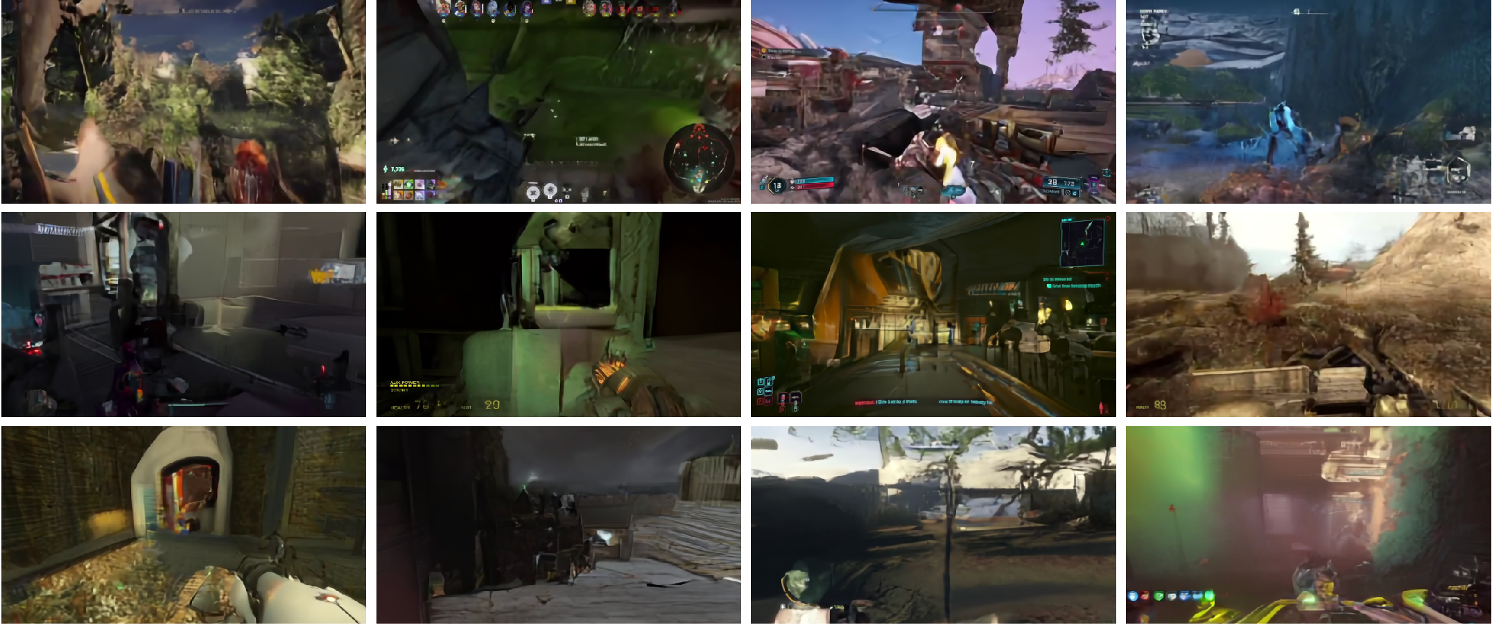
And in our experiments, using transformer based encoders tends to have the same result on downstream generations:

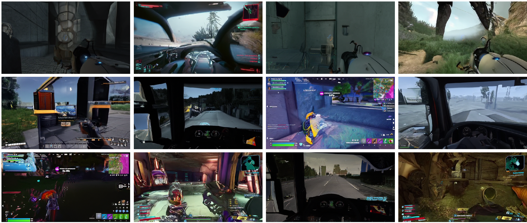
In contrast, see below generated samples in a nearly identical configuration, except with the encoder being a DCAE style resnet:

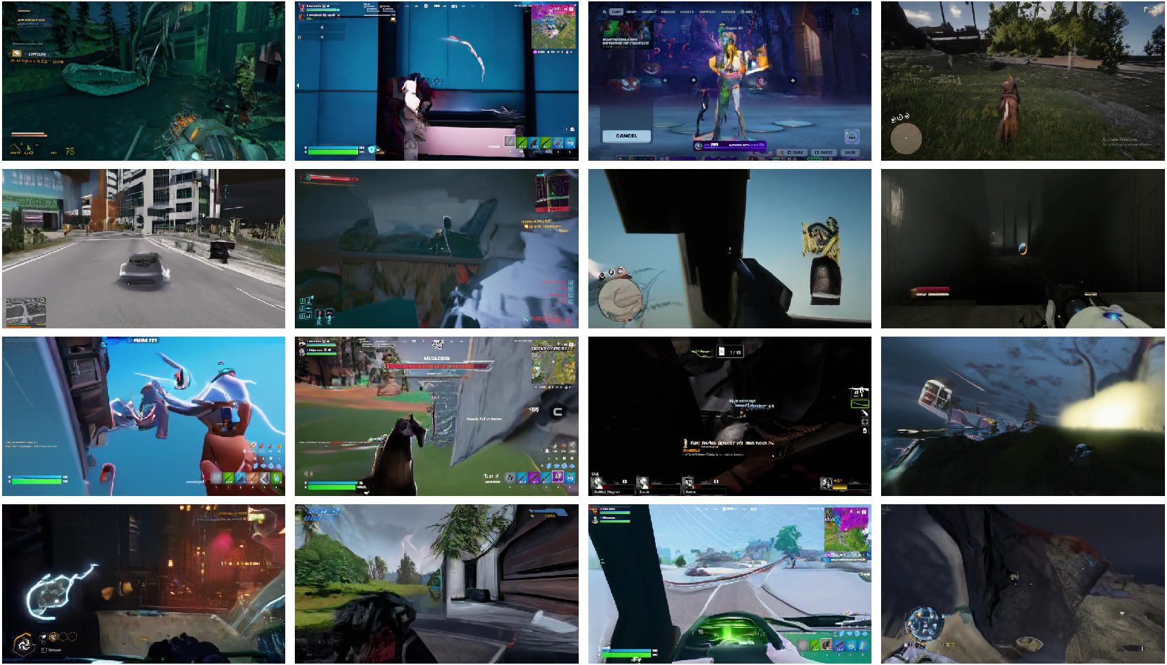
Evidently, the encoder matters far more than the decoder! Which for the above experiments was a transformer itself. We will speak more to the specifics of this later!

GANs Are Hard

One key ingredient on most autoencoder training setups is a GAN loss. But the configurations for this are rarely ever open source. Most large foundation labs fiercely guard specifics on this and do not share it in their papers. This leaves a lot of free variables:

• What discriminator do you use?
• What GAN loss formulation?
• What adversarial weight?
• How do you schedule the adversarial weight?
• How do you balance with other loss terms?

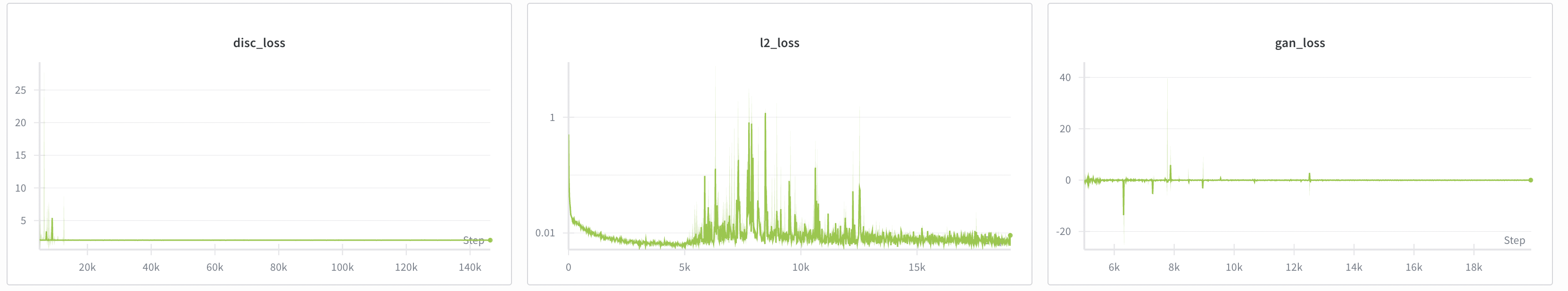
We have only been able to get GAN losses to work under heavily constrained scenarios in which we drop image resolution to 256x256, use a simple PatchGAN discriminator, and use a delayed adversarial weight of 0.25. This is far from ideal as we wanted our decoder to be able to give Waypoint 1 sharp high quality visuals at 360p, and in the future to provide 1080p reconstructions for Waypoint 2. Additionally, landscape aspect ratios are a necessity for game generation. Below is an example of how a good GAN finetuning run went for us:

And then when it doesn’t work… (which was 99% of the time for us):

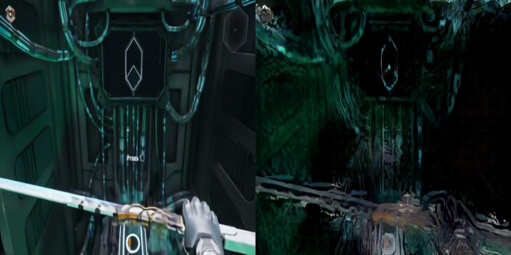
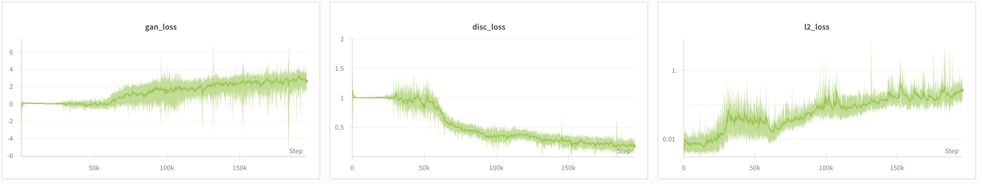
Not ideal!

Diffusion Decoders Are Way Easier

We previously had a blog on diffusion decoders. In our old setup, the encoder was frozen and a decoder (a DiT) was trained given a clean latent and a noisy image. In terms of positional encoding, it saw the input as follows:

Not ideal, and somewhat unnatural in all honesty. It’s as though the latent is some separate image, which it shouldn’t be. As discussed previously, the latent should function as though it were the original image downsampled. Paired with a proxy autoencoder (read the original blog post to know more!) we got some pretty exceptional 1024x1024 samples, even though our latents were only 8x8:

Pretty significant upgrade an MSE+LPIPS decoder:

Note that both decoders used the same encoder, and the same 8x8 latent space.

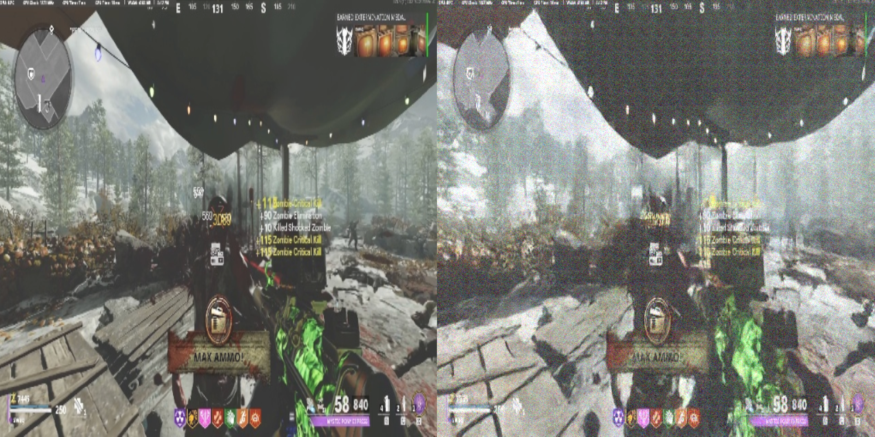
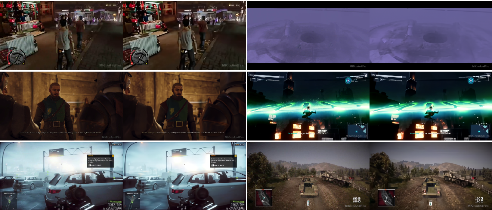
Even though the generation ability of the model was incredible, it often struggled with preserving actual HUD elements, often hallucinating new numbers or details. In this sample you can see how it replaces a few mushrooms with a patch of many small rocks:

Following from this, the generations vary so wildly from frame to frame that trying to use the diffusion decoder on a contiguous video results in something extremely garbled.

Without training the encoder jointly, or doing some form of video-aware training, the encoder has no way of learning to communicate specific details to the decoder, and the decoder has to do a lot of guess-work on what something may have been in the original image. This also hurts its ability to generalize to new data. Notably, our OWL VAE variants (including the Waypoint 1 VAE) work fine on new images that are entirely out of distribution with respect to its training data.

The proxy setup used in our early diffusion decoder experiments also introduced limitations. The diffusion decoder inherited OOD generalization weaknesses from the proxy encoder (in this case the flux autoencoder). There were certain things the proxy autoencoder just did not know how to represent, so the diffusion decoder would always mess them up in its outputs. To solve this, we wanted to follow recent literature showing that diffusion could simply be done in pixel-space. We had very inconsistent results and believed there was a bug in our code, because we kept seeing outputs like this:

We didn’t discover why this was happening until months later.

Back To Basics: X0 Prediction

We eventually realized the reason the diffusion decoder was giving noisy outputs was because of an interaction between the effective dimensionality of the image and the dimensionality of the model. Certain patch size and model dim combos would work while others would not. The effective dimensionality of an image patch is the square of the patch size multiplied by the channel count. For example, with an RGB image using a patch size of 20, the effective dimensionality is 1200. A diffusion model with a dimensionality of 1024 is entirely unable to model the noise and as such it slips through all 50 denoising steps and into the final sample. But… why exactly does an image generation model even need to model noise?

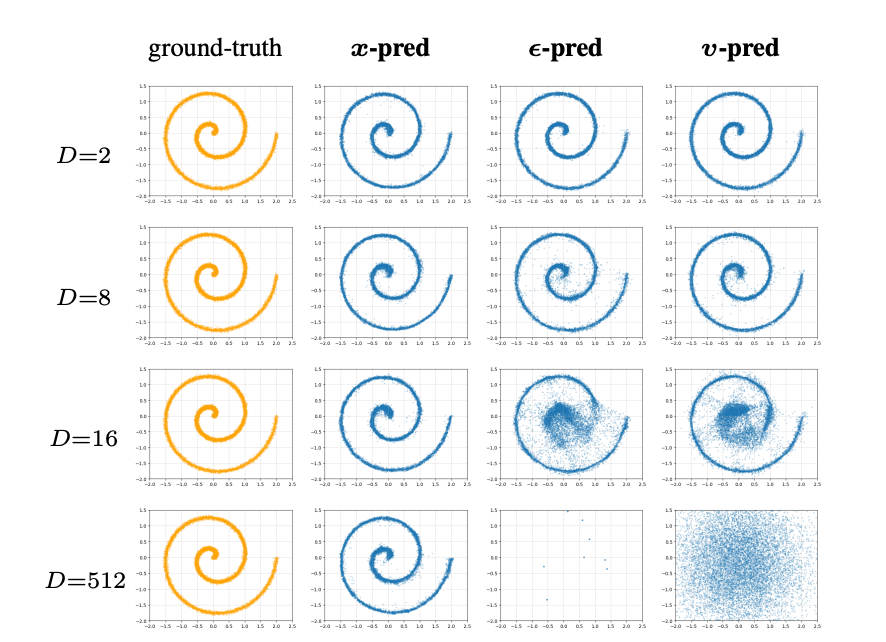
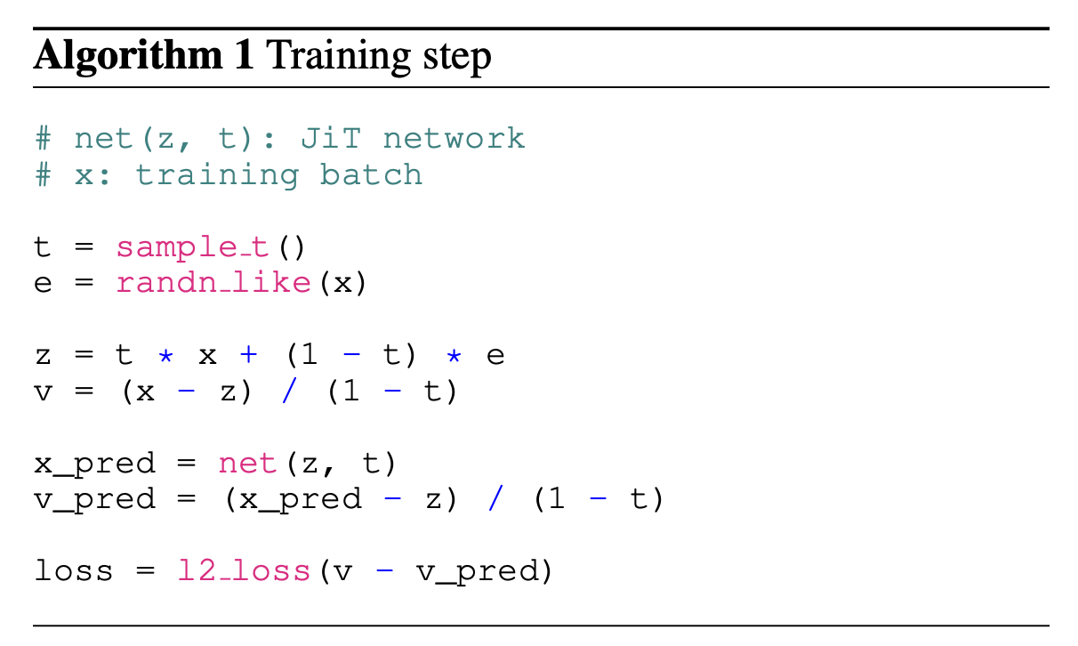
Enter back to basics: a recent paper that showed how, by training diffusion models to output velocity, we are effectively forcing them to learn noise. A flow matching model is trained on a target combining the input image and random noise. Actual images occupy a lower dimensional manifold in a high dimensional space (i.e. the space of actual images is of a lower dimensionality than the space of all possible images including RGB noise). If, per token, the model dim is 1024 and the image dim is 1200, the model has no chance at predicting the target. The paper shows what happens when you do this in a toy domain:

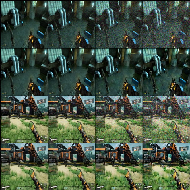
And our experiments show what happens in the pixel diffusion domain:

As a simple solution, reducing effective dimensionality per token below the model dim can actually resolve the issue. This can be done trivially by simply lowering patch size. This was the simplest fix for the problem:

But this is not ideal… halving the patch size quadruples the token count, leading to substantially slower decoding. So what about keeping our larger patch size while using X0 prediction?

So, as we can see, X0 prediction fixes our noise problem from earlier, enabling much larger patch sizes and still producing high quality samples (relative to baseline decoder). Additionally, the model producing the samples above used neighborhood attention with a kernel size of 4. This sparsification reduces VRAM and increases throughput substantially.

We initially wondered if X0 prediction was worth adding to a latent diffusion model, but quickly discovered that the above logic on effective dimensionality is only true for pixel space diffusion. Latent diffusion is robust to noise, so noise carrying through in the denoising process does not matter.

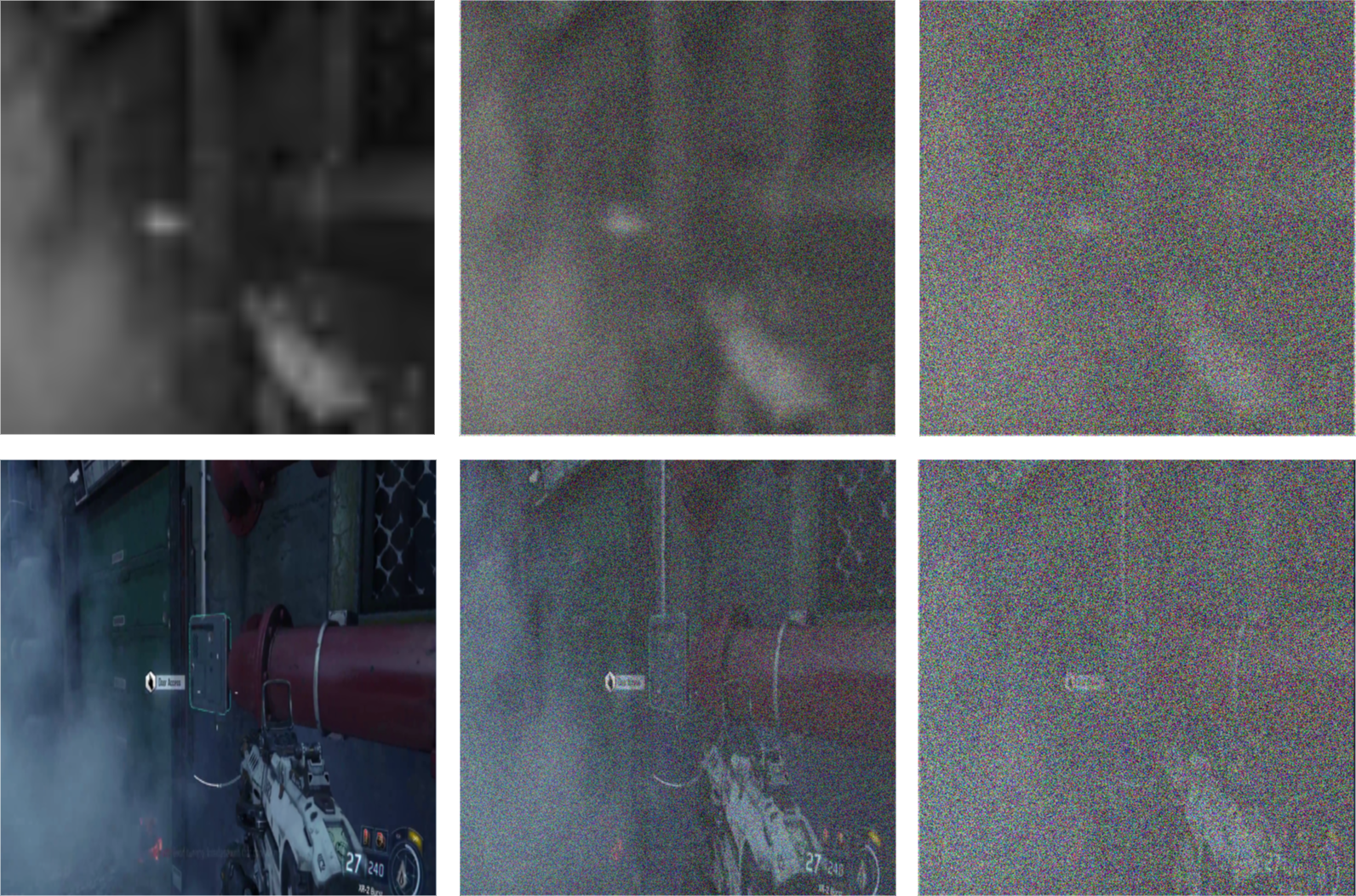
This figure shows the results of noising in pixel space vs latent space. The decoder used in a latent diffusion pipeline actually ends up serving as a denoiser to some extent due to the noising that happens to the latent during VAE training. As such, the noise carried forward during decoding is cleaned out and rendered irrelevant. This leads us to believe that leftover noise in latent diffusion is not a major issue, and that X0 diffusion is primarily only useful in the pixel diffusion domain.

DiTO

Last year you may have seen the paper: diffusion autoencoders are scalable image tokenizers. Diffusion Tokenizers (DiTO) are capable of MUCH higher reconstruction quality than GAN based autoencoders. Given that a 50-step diffusion model has far more GFLOPs to work with, this is rather unsurprising. DiTO is quite different from our prior diffusion decoder work.

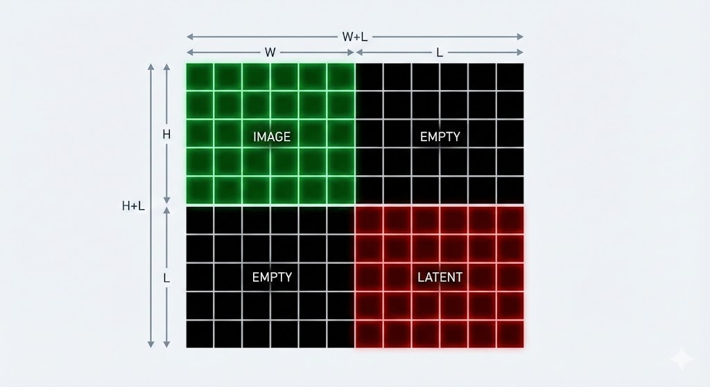
DiTO doesn’t place latents adjacent to images for positional encoding. Latents are instead re-scaled to match image size, then channel-wise concatenated to the image to be denoised.

This ensures spacial correspondence. For the case of a 512x512 image being downsampled to 64x64, you can ensure the top-left-most latent pixel corresponds to the top-left-most 4x4 patch of the original image. You also don’t need to do anything fancy with RoPE since the latent overlays the image! So we have spatial correspondence, what about spectral correspondence? DiTO also does away with KL loss, and presents a novel way to ensure latents are diffusable: noise synchronization.

Normally a diffusion decoder would be given a noisy image and a clean latent, and asked to denoise the image given the latent. With DiTO, the latent is also occasionally noised. When this is done, the image is then noised at least as much as the latent. The idea here is that if you noise the latent 50%, you should noise the image 50% or more. Noising functions as a spectral mask. That is to say, a little bit of noise masks fine details (high frequency), a lot of noise masks coarse details (low frequency). Corresponding noise results in corresponding frequencies.

This ensures denoising is only ever reconstructing details that are still encoded in the noised latent, which subsequently teaches the encoder to produce a latent that can have spectral correspondence with the original image.

DiTO Is Just Better

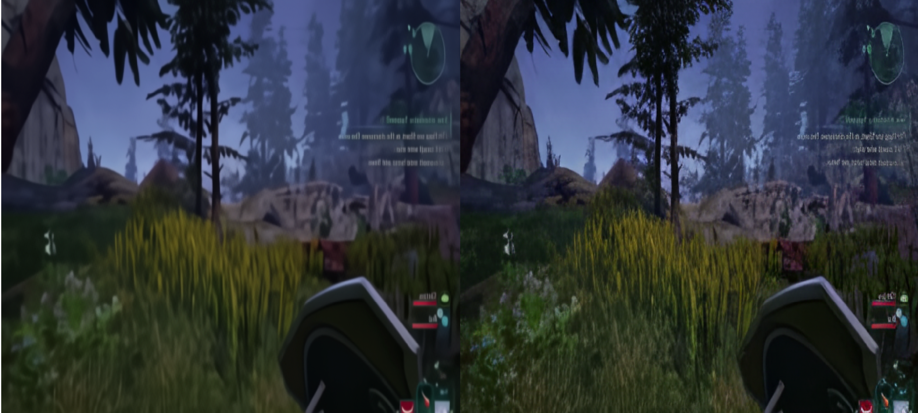
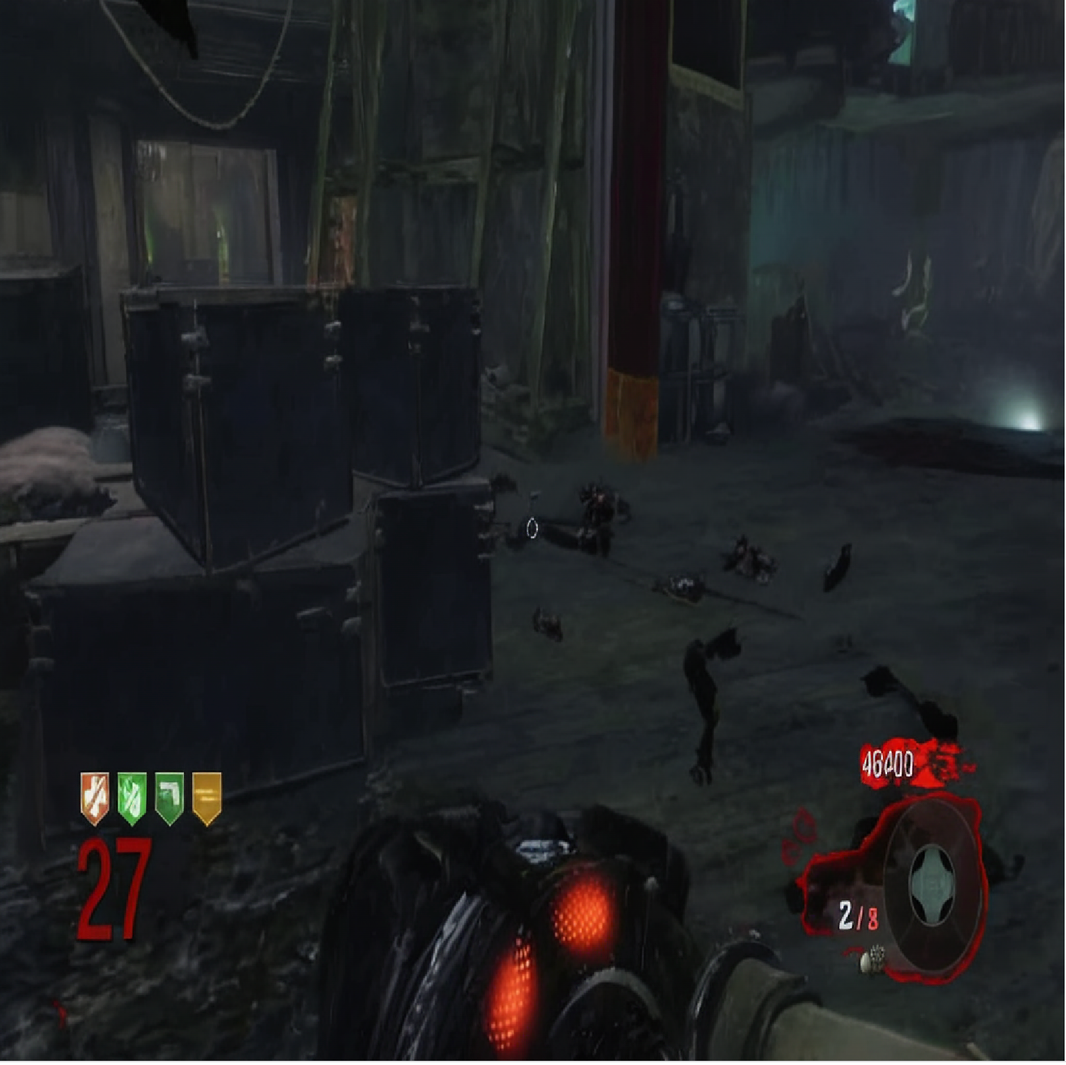
In our experiments, we augment DiTO by using a DCAE encoder to enable deeper compression with higher channel counts, use a DiT instead of a UNet for scalability, use neighbourhood attention, and use x0 prediction to allow for larger patch sizes. The results speak for themselves. First let’s look at the reconstructions from our original f16c16 autoencoder used for Waypoint 1:

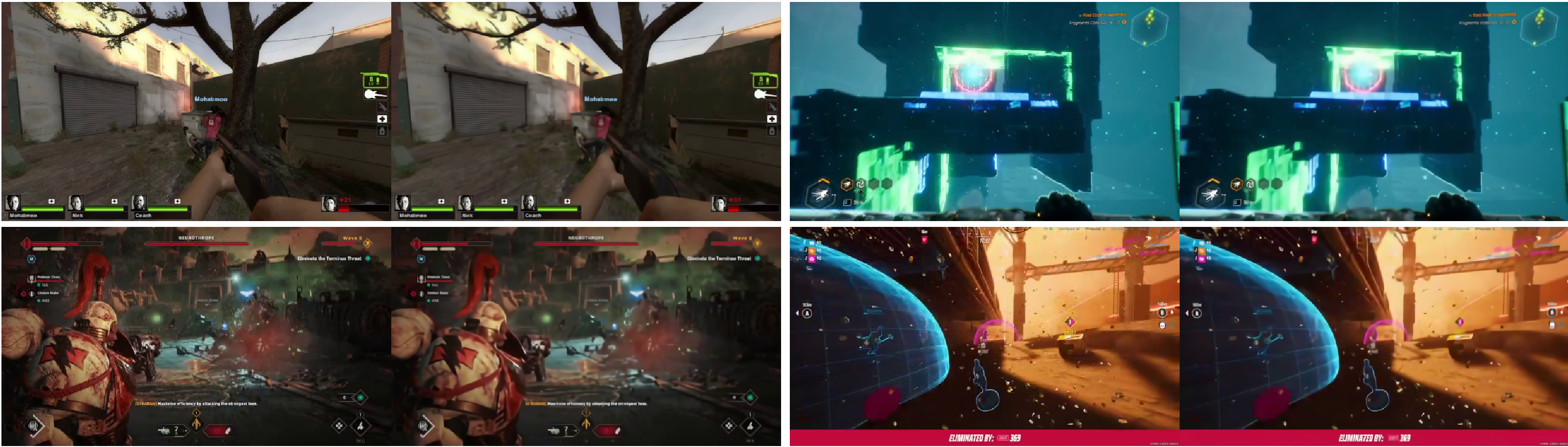
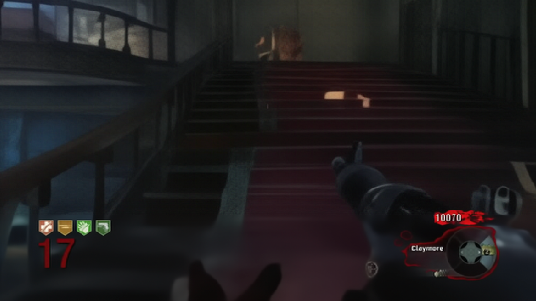
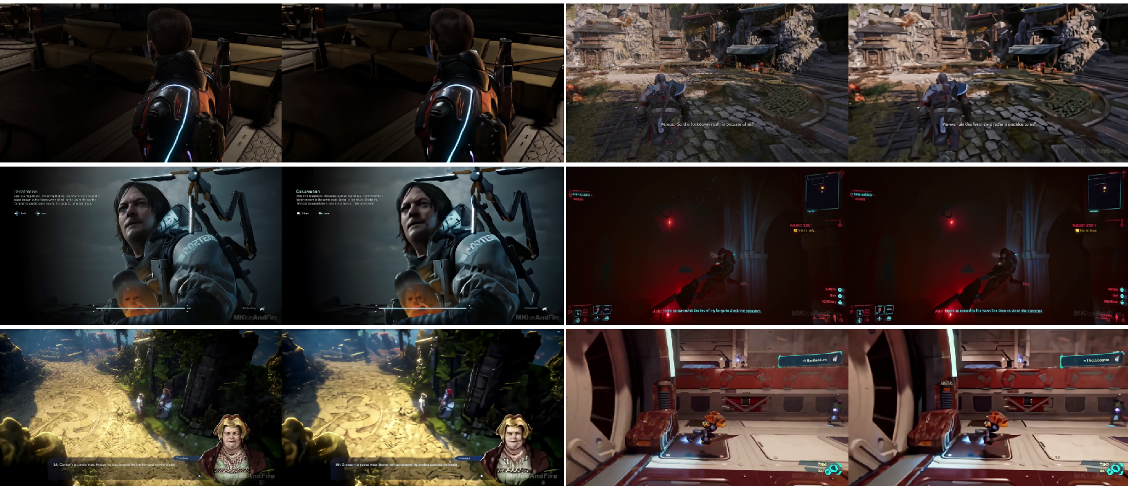
And now a look at the reconstructions from DiTO:

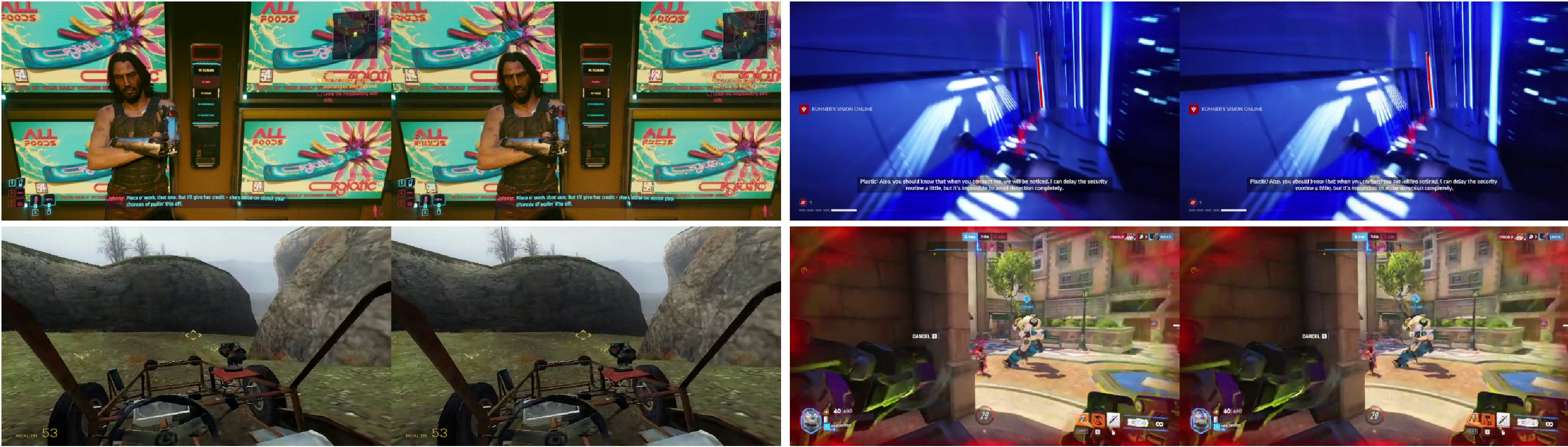
DiTO makes it much easier for the model to learn details like HUD elements and high frequency features like textures on faces, grass, or rocks.

Diffusability

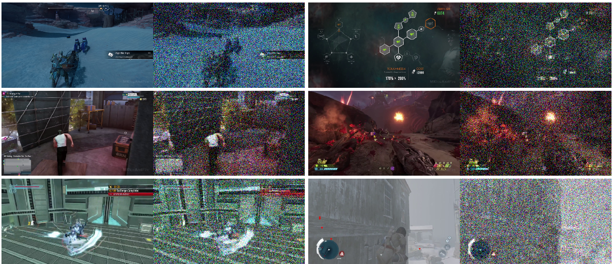
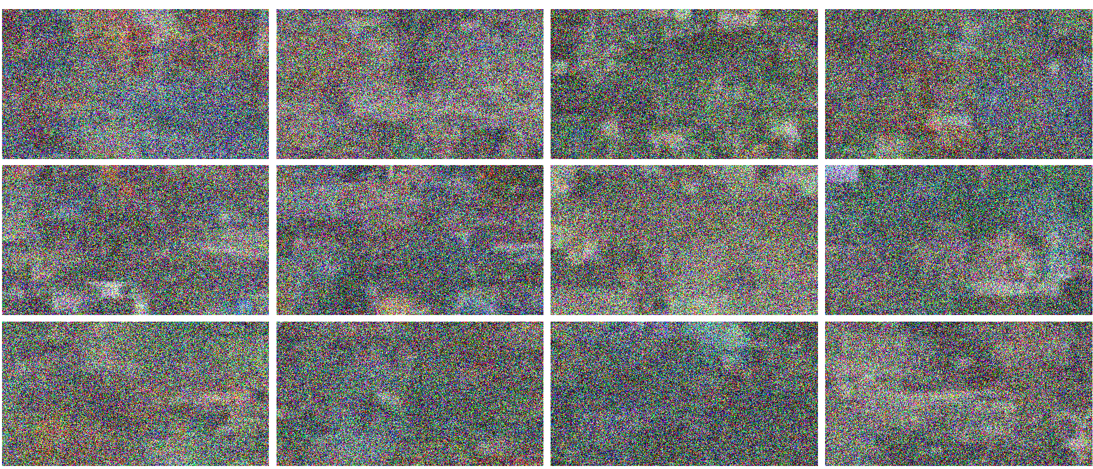
On top of the above, DiTO is very diffusable! Along with this blog post, we are open sourcing OWL Diffusability. As we experimented with novel autoencoder architectures, we found it crucial to assess whether these architectures were satisfactory for downstream latent diffusion training. Rather than doing large world model training runs, we instead zoomed in on unconditional image generation. We now train a small DiT up to 30,000 steps on our Waypoint 1 dataset, aiming to get about 256 tokens per image to get GFLOPs constant. We (unsurprisingly) found that pixel diffusion doesn’t work with a high patch size using v prediction:

With x0 pred, it works but isn’t very good past 256x256 (that is to say, latent diffusion is still absolutely preferred):

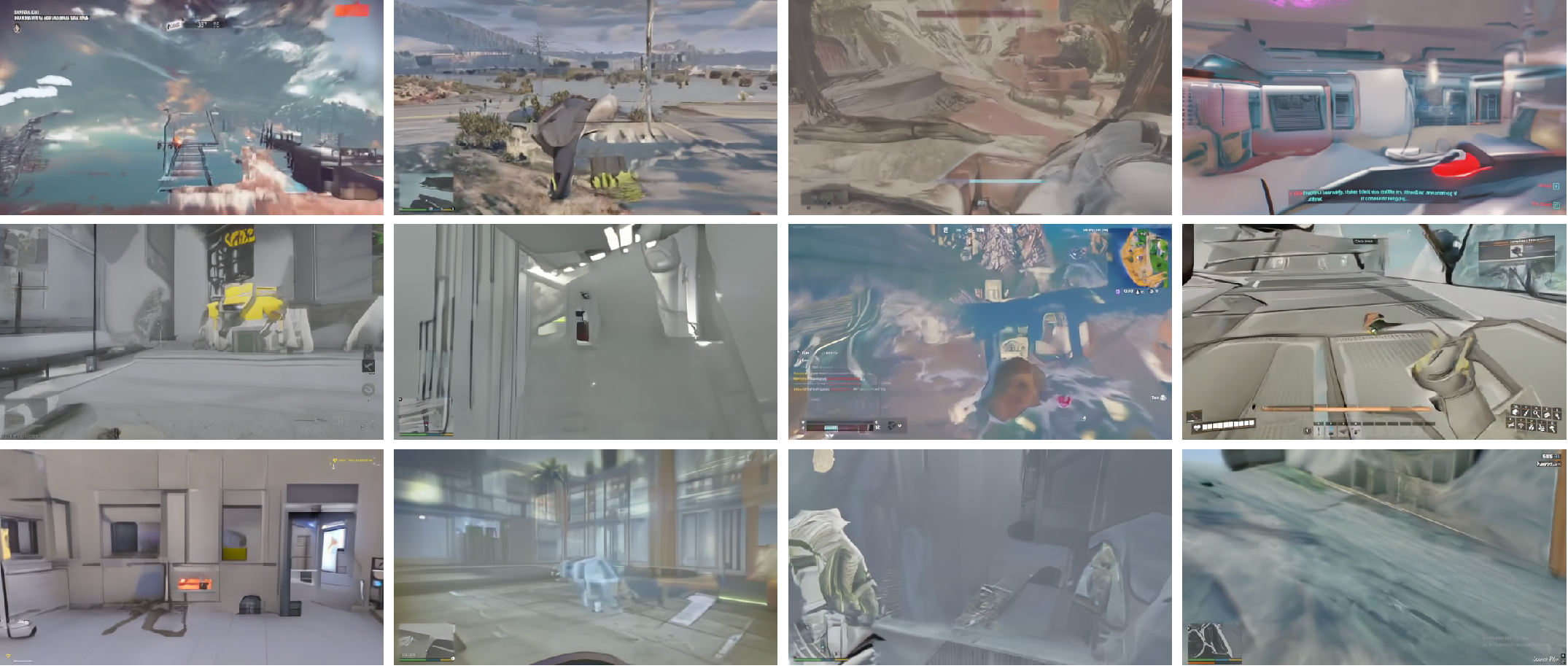
We found that the original Flux 1 VAE works but is not ideal for fast training:

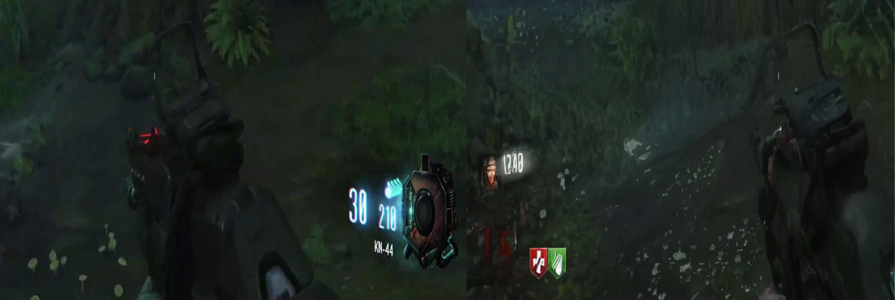
On the other hand the Waypoint 1 f16c16 VAE works great! But is a little blurry…

The DiTO f16c16 VAE is even better (and much sharper):

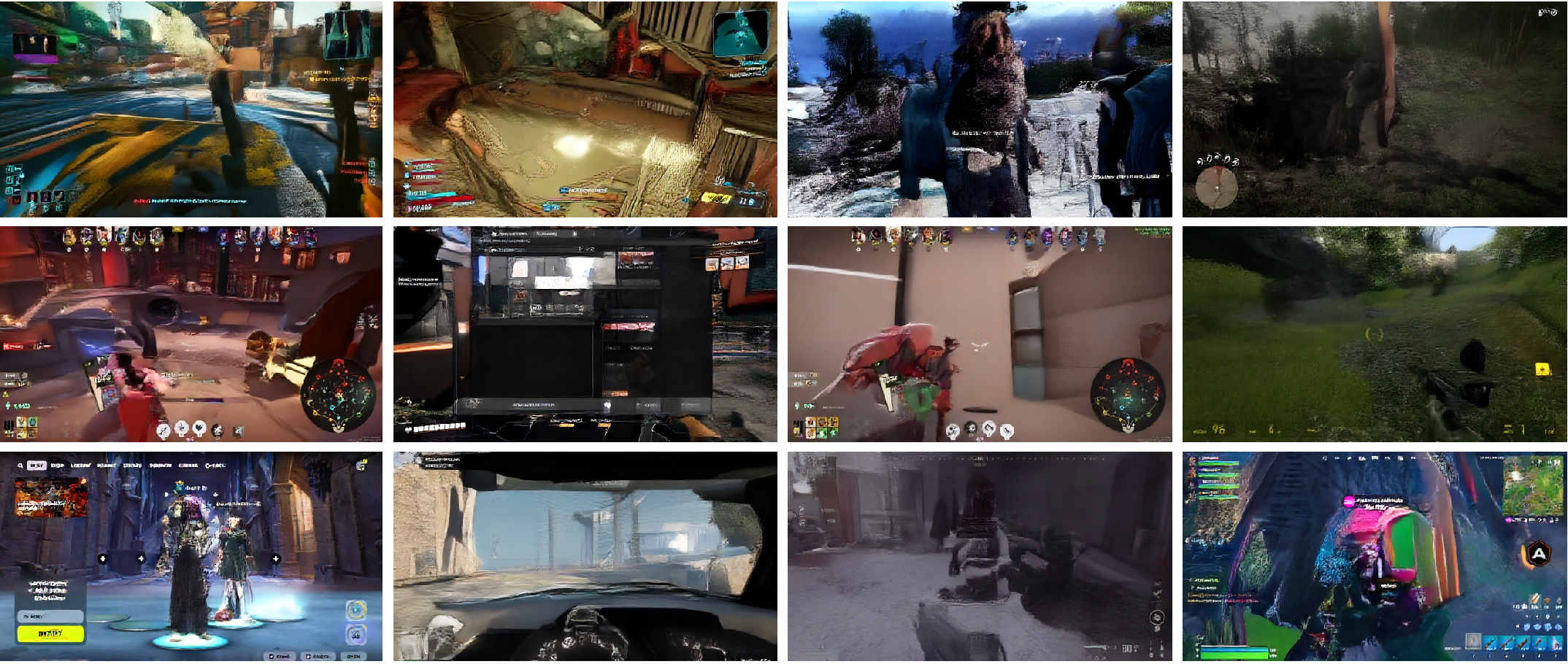
And finally, we also tried a transformer encoder for DiTO, which produced better reconstructions, but seems to be significantly less diffusable.

This gave us the insight that the encoder often matters more for diffusability than the decoder, supporting our choice of maintaining a DCAE resnet encoder with a transformer based diffusion decoder.

VideoDiTO

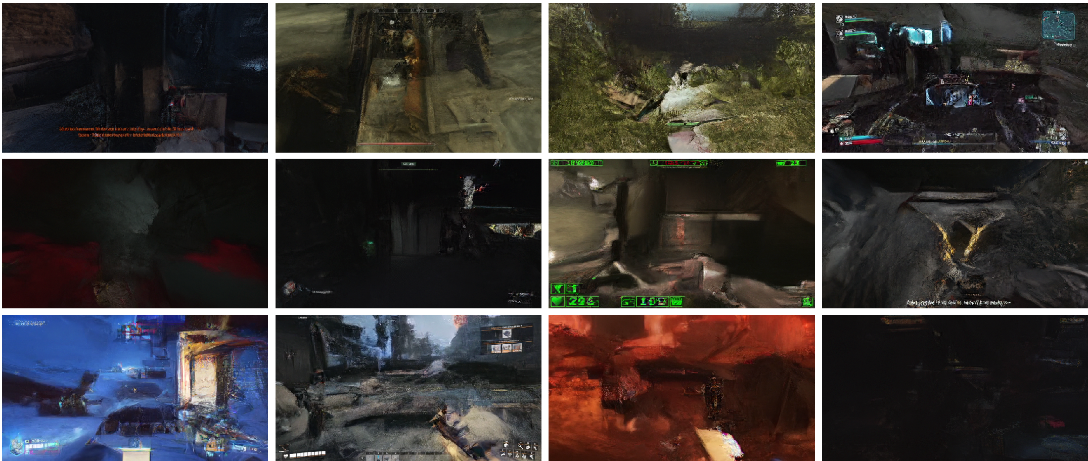
Naturally the next step was trying DiTO for video compression with a temporal compression factor. In our initial experiments this was extremely unstable, and we were unable to train any model without a complete collapse in training past 10,000 training steps:

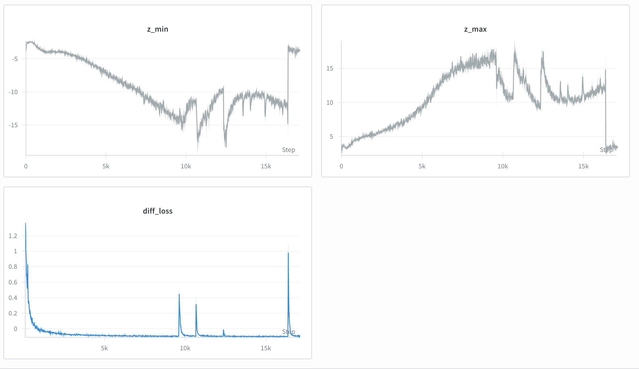
After extensive debugging, we found that this was actually due to the target generation in x0 prediction:

In pixel space, it is more important for the model to get high frequency features correct, to avoid high frequency noise corrupting the samples. For this, the original paper proposes transforming the target and prediction before MSE loss in order to re-weight the objective. We discovered that this division leads to extreme instability when you start to increase the batch size or sample size. With videos, we noise each frame to a different noise level. This means we are sampling many more timesteps, so the odds of getting an unstable timestep in any given training step is much higher. By simply removing this rescaling and training the model to directly regress output to the original image (x), we were able to entirely solve instability and get ourselves a video diffusion autoencoder with 4x temporal compression. This model still needs to be scaled, and made causal (to encode/decode long videos), but it’s a good first step!

Why?

Diffusion autoencoders are far easier to train than a GAN VAE. They also have some interesting properties we’re hoping to leverage for Waypoint 2. Particularly, one can directly control how much the latent influences the reconstruction using guidance and latent noising, actively controlling the trade-off between reconstruction and generation at inference-time. Combined with text conditioning, we are aiming to use this for live restyling. This would enable one to play a World Model game and actively go between a cel-shaded style, a photorealistic style or an anime style for example. This kind of setup positions the world model as the simulation engine and the decoder as the actual renderer. In the near future, we hope to share more work in this direction!

Outro

We think that diffusion tokenizers are a tangible path towards HD, diffusable, and controllable, video representations. DiTO gives us a decoder that is more expressive, and still compatible with diffusion training. That being said, there are some hurdles that still need to be overcome, hence why we are not actively using them in our world models. These autoencoders are significantly slower than a one step resnet decoder, and many optimizations will be needed to make them fast enough to run smoothly.

Next week we’ll talk a bit more about the prompting pipelines we are using to improve Waypoint 1, and the path we are taking towards Waypoint 1.5, our next major release. If you want to be a part of how world models evolve, see results as they land, or follow along as we ship this work in real time, join the Overworld Discord, or play the most recent build of the model.